CANDID

CANDID - “Complete And Noiseless Distributions from Incomplete Data”.

A flexible expectation-maximisation (EM) method that implements and builds upon the principles of Extreme Deconvolution (Bovy+11).

Unlike PyGMMIS, CANDID’s intended purpose is the full modelling of highly multi-dimensional galaxy property distributions when the data are missing are biased - an outstanding problem in astronomy with no one easy fix.

CANDID deals with the following issues, many of which have known solutions, just not ones that are implemented together.

1. Heteroscedasticity

   It is common for each data point to have its own uncertainty distribution. Moreover, the size of the uncertainty distribution frequently changes across the parameter space. In the fitting of simple models, heteroscedasticity is incorporated naturally with the addition of a \(\chi^2\)-like term into the likelihood. Extreme Deconvolution handles heteroscedasticity.

2. Non-Gaussianity

   Assuming a Gaussian error distribution dramatically simplifies the posterior and hence the analysis. However, the Gaussian assumption is frequently incorrect and may lead to dramatically misleading results. For example, the uncertainty distribution of a flux measurement is easily approximated as Gaussian but given that the intrinsic value is strictly positive, this assumption breaks down at low signal-to-noise. resamples the uncertainty distribution of each data point consistently such that flux variables remain strictly positive. The Gaussian mixture EM algorithm can readily be extended to incorporate resampled data points instead of directly solving for the convolution of the data uncertainty and model components. resampled data).

3. Incompleteness

   It is not possible to rerun the universe nor observe the entirety of a population in astronomy. Typically, incompleteness is addressed by methods such as \(1/V_{max}\) or Monte Carlo simulations of point sources given an error map. However, when the number of dimensions grows, what is applicable to each variable individually becomes complicated when considering their covariation. aims to deal with incompleteness naturally by “imputing” the missing values from the approximated observed model given known selection criteria, following PyGMMIS.

4. High dimensionality

   The “curse of dimensionality” firmly applies to Gaussian mixture models since each Gaussian component contributes \(d(d+1)/2 + d + 1\) dimensions to the likelihood from its covariance matrix, mean vector and weight relative to the other components. Rejection sampling MCMC techniques start to fail at tens of parameters and interpolating ensemble MCMC (such as emcee) fails at hundreds of parameters. The EM algorithm is well suited to finding the peak of the posterior distribution. By dropping the need to sample the entire posterior distribution, we can iterate towards the maximum likelihood peak and then bootstrap, if need be, to sample its width.

I have recently been applying CANDID to the LOFAR LoTSS DR1 data in the hopes of validating the mass dependency found in the \(SFR-L_{150MHz}\) relation (Gurkan+18).

This is a complex dependency since the shape of the \(SFR-L_{150MHz}\) relation could non-linearly depend on redshift and mass. In addition, there are complex selection effects to be taken into account: magnitude r-band limit with SDSS, BPT emission line selection with MPA-JHU data, and a redshift limit.

That’s 9 dimensions, which equates to \(N = kd(d+1)/2 + kd + (k-1)\) parameters for the model, where \(k\) is the number of component Gaussians and \(d\) is the number of dimensions.

But it appears to work! Look below for the full corner plot of our 9-dimensional space.

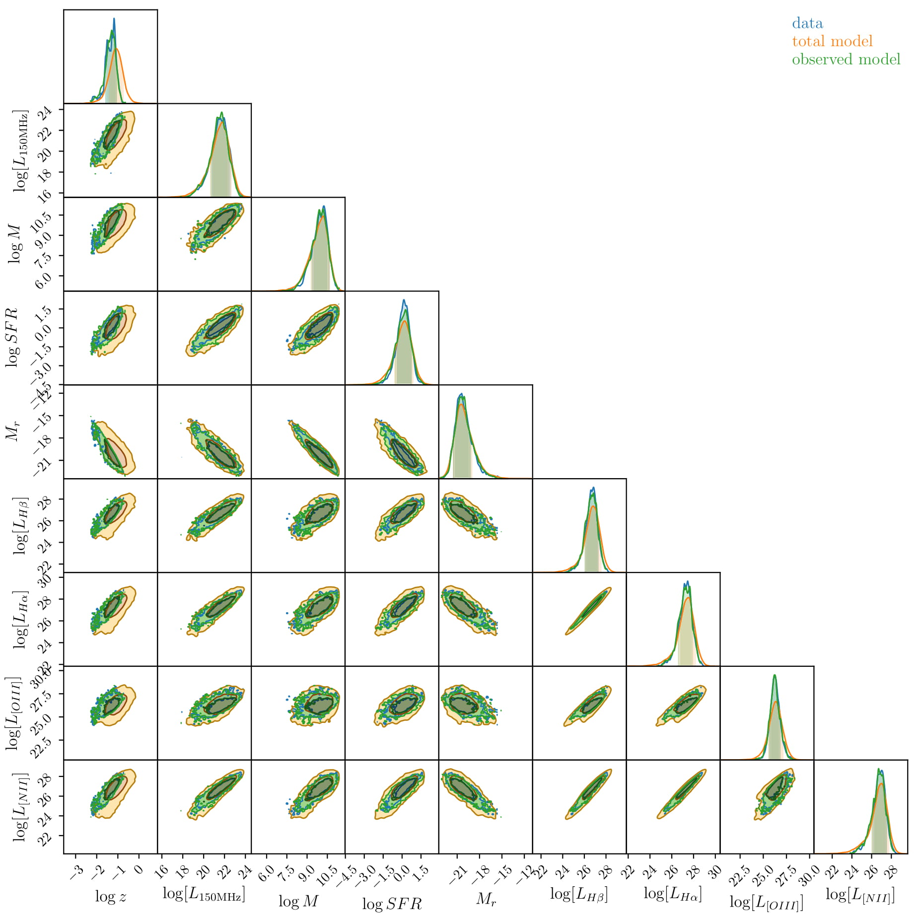
The yellow is our model of what the data would look like in the absence of obscuration or selection effects, the blue is the actual observed data, and the green (which is hard to see because it matches the blue so well!) is our prediction for the data when the selection effects are applied!

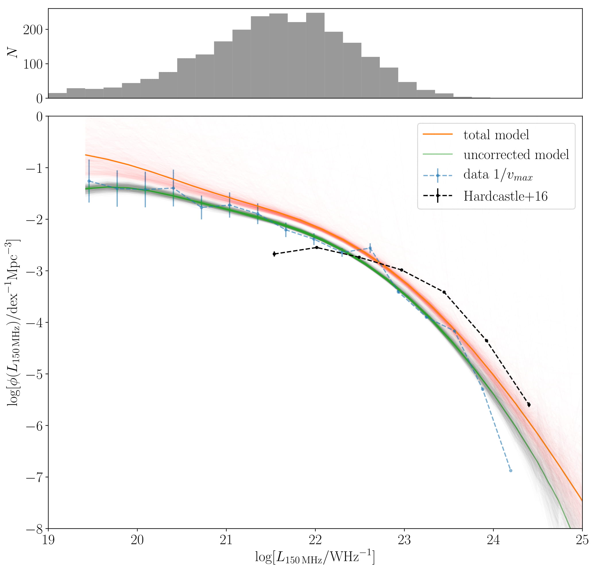
Here I have used 9 component Gaussians (set by some very simple Bayesian Information Criterion tests) so this is 548 parameters we are fitting. To include all the uncertainties (which themselves are not Gaussian), would take fair bit of cluster time. So for the purposes of demonstration I have simply bootstrapped the model over realisations of the data drawn from their uncertainty distribution. This has the effect of broadening the posterior distribution and so when we estimate uncertainties on our products, they are quite large. This can be fixed easily, just need to write in the Extreme Deconvolution aspect! You can see the bootstrapped realisations in the extracted luminosity function, below.

It is possible to slice through this 9-dimensional model and extract any relation you like. Here we have marginalised over the redshift-luminosity plane (since our model consists only of Gaussians, this 2D marginalisation will also consist of Gaussians!). Then its a simple step to turn \(L_{150}-z\) into a traditional luminosity function. The one shown below is the total for \(0.004 < z < 0.25\), but we could just as easily specify one at exactly \(z=0.1\).

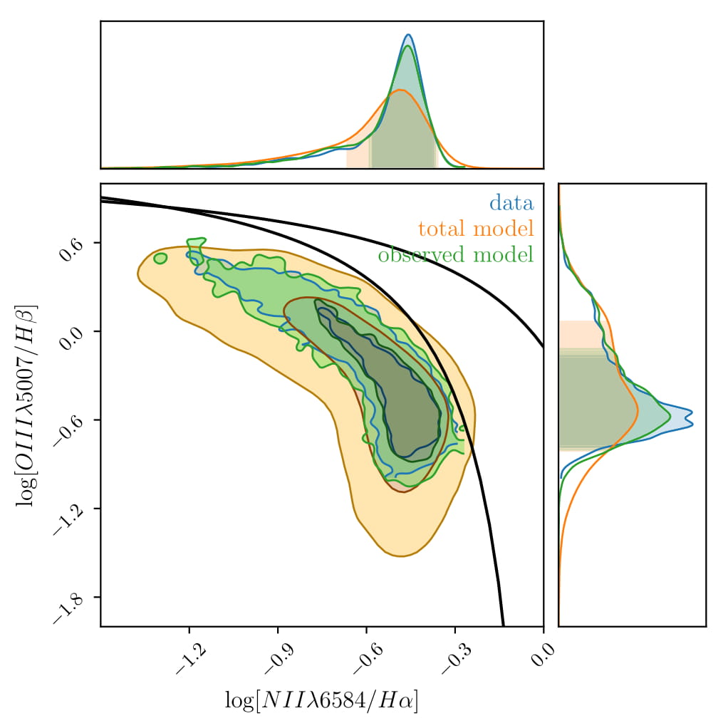
We can see already that composite relations extracted from the model, such as BPT fit the data really well. Despite the fact that the model is not aware of BPT diagrams (it is only given the emission line luminosities), it captures its shape very well.

Below, we can see that the magnitude distribution of the data is recreated.

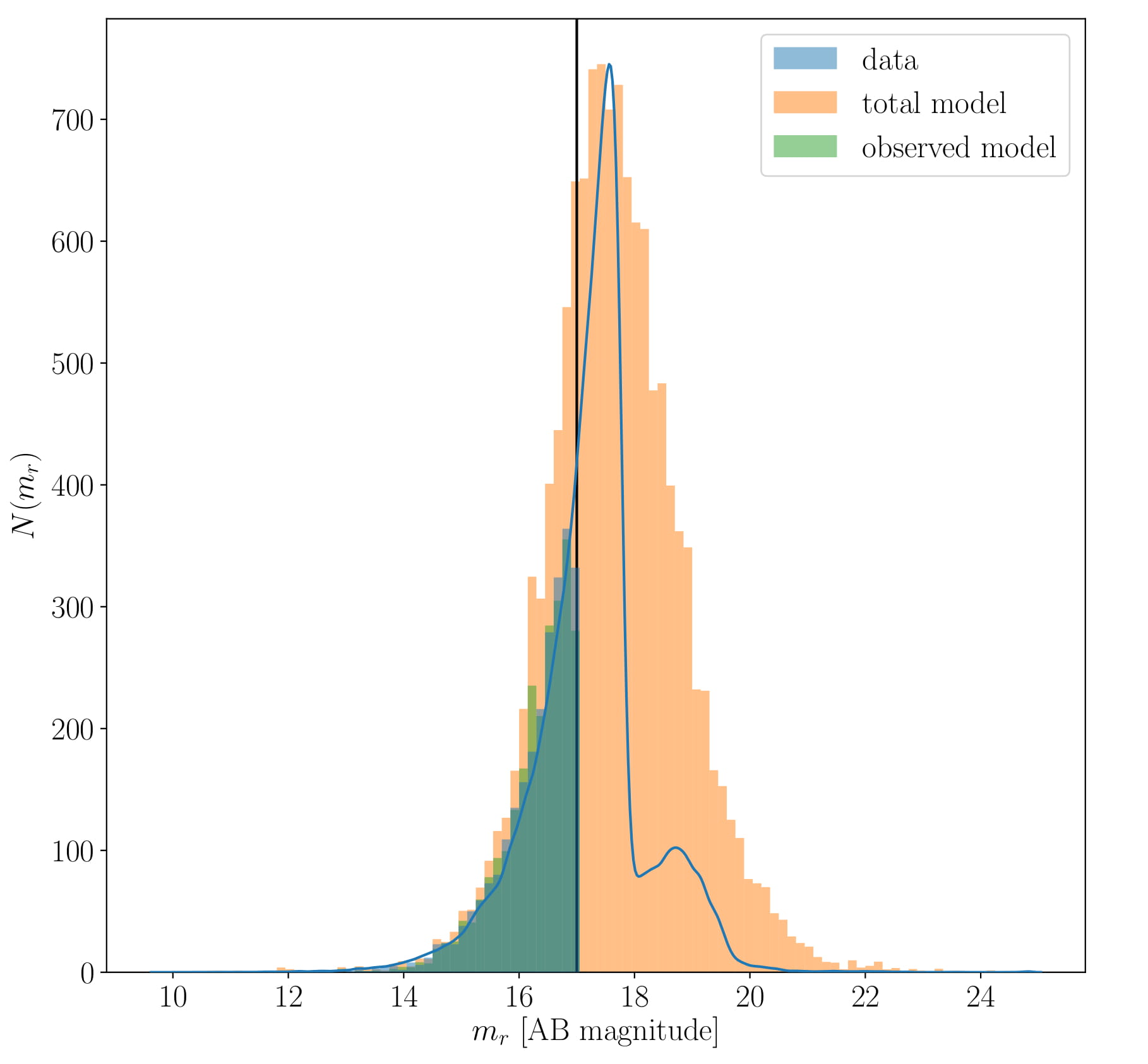
The blue line shows the full SDSS catalogue (not just the Gurkan+18 dataset, which is shown as the blue histogram) and you can see that the model can reproduce the shape and peak of the distribution, as well as indicating that there are galaxies missing due to non-magnitude-limit effects.

All of this works because expectation-maximisation guarantees a likelihood increase¹. However, since the errors in luminosity are definitely not Gaussian at low luminosity, and that we’re fitting the Gaussians in log-space, and that we are imputing the missing samples to infer the missing distribution, we have to iterate stochastically.

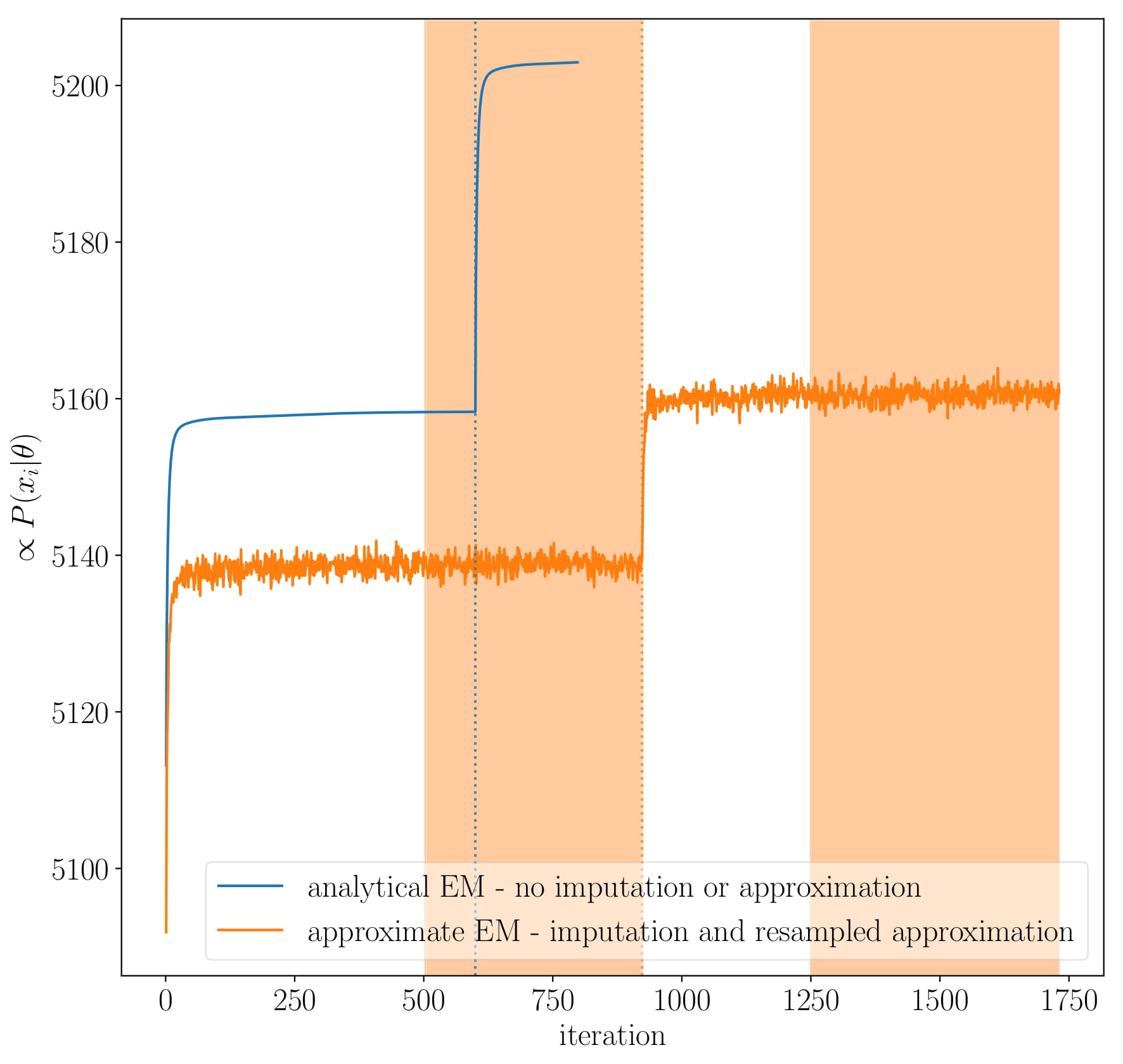
The blue line in figure above shows the traditional EM algorithm always increasing the likelihood with each step. The orange line indicates our stochastic approach. Here, the likelihood can decrease because we’re approximating the likelihood but it will be stable around that approximation. This means that we can expect increase in likelihood when the noise in the approximation is not too much - i.e. when EM strays too far away from the analytical solution, the current iteration is evaluated as too bad and so it shoots back, creating a cycle.

The result is a holistic model which the user can step through and manipulate with ease!

There are so many more things I want to do with this:

• Implement extreme deconvolution properly
• Experiment with slice sampling instead of EM (could be a headache)
• If I can make slice sampling/some Bayesian sampler that can handle >500 parameters work here, then it would be simple to add analytical constraints. For instance, it would be possible to construct the same non-parametric model as above but constrain the luminosity function to be a Schechter function.

This is very much a work in progress! The github repo is private for now until I have cleaned it up a bit!

^{1Technically it only guarantees a likelihood that doesn’t decrease and so it can get stuck in local maxima. However, we can get round this with bootstrapping initialisation and the “split-and-merge” algorithm.}